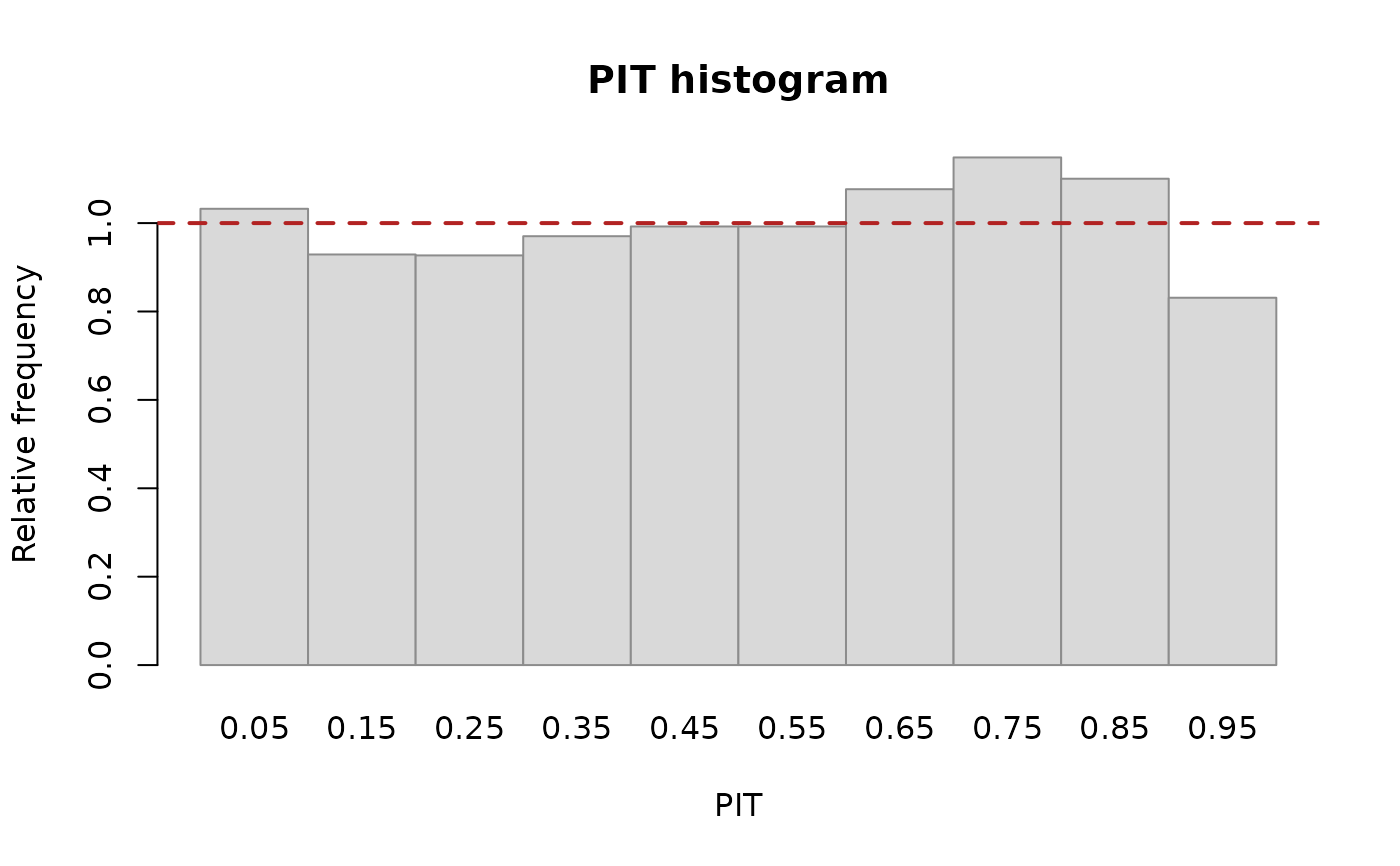
Non-randomized PIT histogram for a fitted count model

Draws the non-randomized probability integral transform histogram of Czado, Gneiting, and Held (2009). A well-calibrated model yields a flat histogram at height one (the reference line); a U shape indicates under-dispersion in the predictive distribution and a hump indicates over-dispersion.

Usage

pit_hist(
  fit,
  bins = 10,
  main = "PIT histogram",
  xlab = "PIT",
  ylab = "Relative frequency",
  ...
)

Arguments

fit: A fitted underdisp count model (any class score() takes); a fit with frequency weights counts each row as many times as its weight.
bins: Number of histogram bins.
main, xlab, ylab: Plot labels.
...: Passed to graphics::barplot().

Value

Invisibly, the vector of bin heights (normalized so that a calibrated model gives heights near one).

Examples

set.seed(1)
y <- rcpb(400, lambda = 3, alpha = 0.5)
fit <- cpb(y ~ 1, data = data.frame(y = y), truncated = FALSE, se = "none")
pit_hist(fit)