Hanging rootogram for a fitted count model

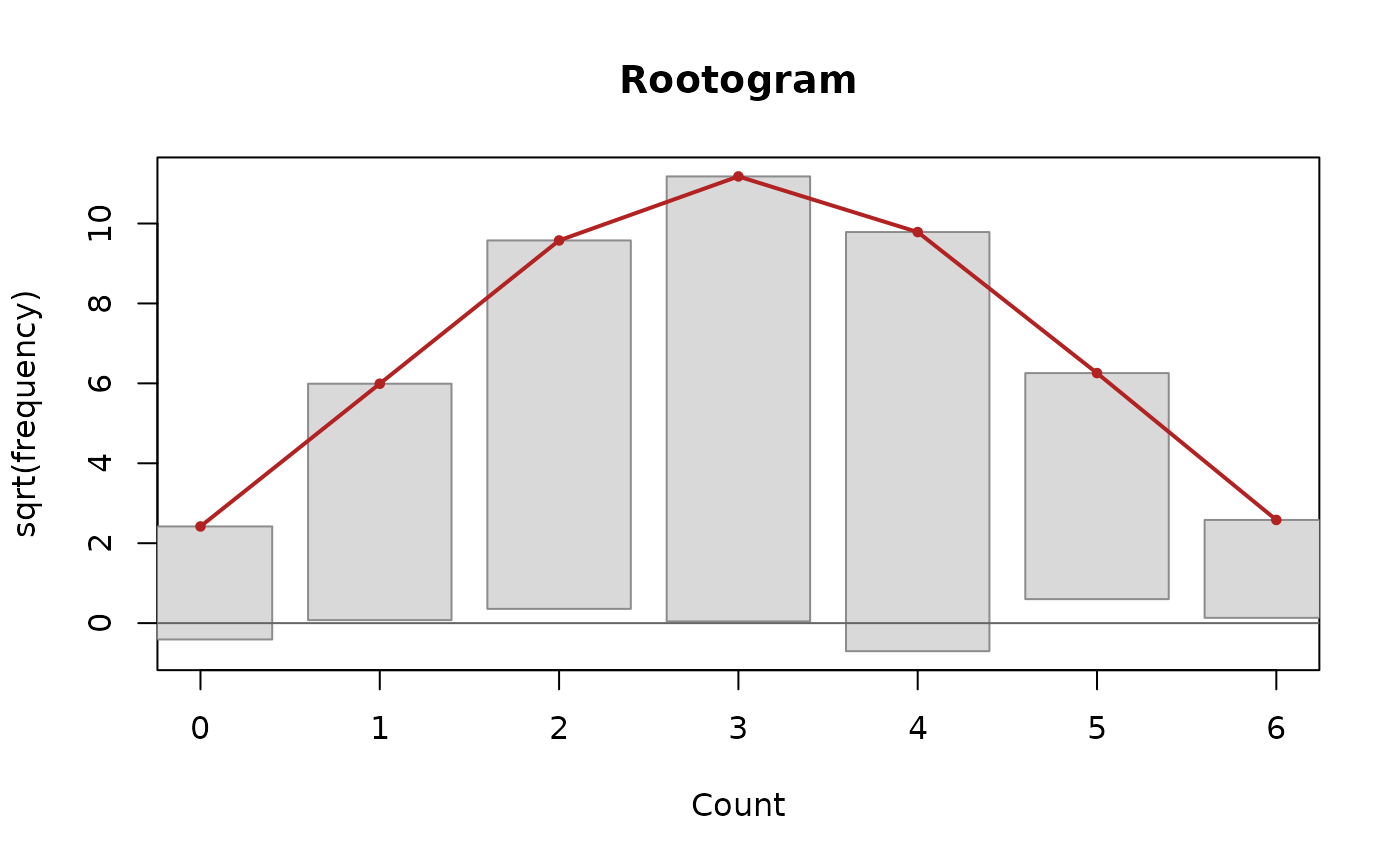
Draws a Tukey hanging rootogram: bars for the observed frequencies hang from the curve of expected frequencies, both on the square-root scale. Bars that hang below the zero line mark counts the model under-predicts; bars that stop short mark counts it over-predicts. A fit with frequency weights counts each row as many times as its weight in both the observed and the expected frequencies.

Usage

rootogram(
  fit,
  kmax = NULL,
  main = "Rootogram",
  xlab = "Count",
  ylab = "sqrt(frequency)",
  ...
)

Arguments

fit

A fitted underdisp count model (any class score() takes).

kmax

Highest count to display; defaults to the maximum observed count.

main, xlab, ylab

Plot labels.

...

Passed to graphics::plot().

Value

Invisibly, a data frame of count, observed, and expected frequencies.

Examples

set.seed(1)
y <- rcpb(400, lambda = 3, alpha = 0.5)
fit <- cpb(y ~ 1, data = data.frame(y = y), truncated = FALSE, se = "none")
rootogram(fit)