Predicted probabilities, first differences, and marginal effects

An inflated ordered model has more moving parts than a plain ordered model: category probabilities, regime probabilities, and the posterior probability that an observation in the inflated category is an inflated case, each of which can change when a covariate moves in one equation, the other, or both. This vignette walks through the tools that turn a fit into those quantities and into tables and figures. The running example is the zero-inflated ordered probit of political violence from vignette("iop"):

library(iop)
data(bp)
m <- iop(violence ~ loggdppc + parliament + disaster + major_oil + major_primary |
           loggdppc + parliament + disaster + major_oil + major_primary,
         data = bp, inflate = "bottom")

Everything below works the same way for oprobit(), ologit(), and iol() fits; the regime-related quantities are simply absent (or equal to one) for the uninflated models.

Predicted probabilities

predict() has one type per quantity:

`type`	Returns
`"prob"` (default)	the n x J matrix of category probabilities P(y = j)
`"class"`	the modal category
`"prob_outcome"`	the ordered-stage probabilities P(y = j \| ordered regime)
`"regime"`	P(ordered regime)
`"inflated"`	P(inflated regime) = 1 - P(ordered regime)
`"posterior"`	P(inflated regime \| y = inflated category), 0 for other categories
`"prob_conditional"`	for random-intercept fits, P(y = j) at a zero random intercept
`"link"`, `"link_inflation"`	the two linear predictors

head(predict(m), 3)
#>           none  repression   civil war
#> [1,] 0.9674842 0.022065503 0.010450287
#> [2,] 0.9822735 0.008319777 0.009406761
#> [3,] 0.9769820 0.015619602 0.007398424
head(predict(m, type = "class"), 3)
#> [1] none none none
#> Levels: none repression civil war
head(predict(m, type = "prob_outcome"), 3)
#>           none repression civil war
#> [1,] 0.5840688  0.2822546 0.1336766
#> [2,] 0.2712834  0.3420160 0.3867006
#> [3,] 0.5840193  0.2822768 0.1337040
summary(predict(m, type = "regime"))
#>      Min.   1st Qu.    Median      Mean   3rd Qu.      Max. 
#> 1.641e-05 7.771e-01 9.947e-01 7.927e-01 1.000e+00 1.000e+00

The posterior probability separates, among the observed zeros, those the model attributes to the inflated regime (structurally peaceful country-years) from those it attributes to the ordered regime (at-risk country-years that stayed calm):

post <- predict(m, type = "posterior")
summary(post[bp$violence == "none"])
#>      Min.   1st Qu.    Median      Mean   3rd Qu.      Max. 
#> 0.000e+00 7.300e-07 3.021e-02 2.896e-01 6.880e-01 1.000e+00

The two types of zeros

Harris and Zhao (2007) decompose the probability of the inflated category into its two sources: type = "zeros" returns, for every observation, the mass that arrives through the inflation process ( $1 - P(s = 1)$ , the structurally peaceful) and the mass that arrives through the ordered stage ( $P(s = 1, y^* = k)$ , at-risk country-years that stayed calm); the two columns sum to $P(y = k)$ :

z <- predict(m, type = "zeros")
head(cbind(z, total = rowSums(z), P_none = predict(m)[, "none"]), 3)
#>      inflation     ordered     total    P_none
#> [1,] 0.9218241 0.045660092 0.9674842 0.9674842
#> [2,] 0.9756743 0.006599157 0.9822735 0.9822735
#> [3,] 0.9446656 0.032316328 0.9769820 0.9769820
colMeans(z)
#> inflation   ordered 
#> 0.2072868 0.5098365

first_difference() and ame() report effects on both components with decompose = TRUE, which is how Harris and Zhao present the marginal effect on the zero probability:

first_difference(m, "loggdppc", from = 7, to = 9, decompose = TRUE)
#> First differences: loggdppc from 7 to 9 [at the typical profile]
#>               component  from    to   diff  lower upper method
#>             P(y = none) 0.645 0.781  0.136 -0.080 0.351  delta
#>       P(y = repression) 0.253 0.156 -0.097 -0.251 0.058  delta
#>        P(y = civil war) 0.102 0.063 -0.039 -0.102 0.024  delta
#>       P(ordered regime) 1.000 0.616 -0.384 -1.012 0.243  delta
#>  P(y = none: inflation) 0.000 0.384  0.384 -0.243 1.012  delta
#>    P(y = none: ordered) 0.645 0.396 -0.249 -0.672 0.175  delta

Two further summaries are type = "mean" (the expected category index $\sum_j j\,P(y = j)$ on the 0, …, J-1 scale) and type = "cumulative" ( $P(y \le j)$ ).

Covariate profiles and standard errors

newdata takes any data frame with the model’s covariates, and se.fit = TRUE adds delta-method standard errors for every probability type:

nd <- data.frame(loggdppc = c(6, 8, 10), parliament = 0, disaster = 0,
                 major_oil = 0, major_primary = 0)
p <- predict(m, newdata = nd, se.fit = TRUE)
round(p$fit, 3)
#>       none repression civil war
#> [1,] 0.689      0.229     0.082
#> [2,] 0.689      0.229     0.083
#> [3,] 0.990      0.008     0.003
round(p$se.fit, 3)
#>       none repression civil war
#> [1,] 0.028      0.017     0.014
#> [2,] 0.021      0.015     0.009
#> [3,] 0.011      0.008     0.003
predict(m, newdata = nd, type = "inflated", se.fit = TRUE)
#> $fit
#> [1] 4.629630e-13 4.038893e-03 9.673703e-01
#> 
#> $se.fit
#> [1] 3.742466e-12 9.159496e-03 3.618732e-02

First differences

first_difference() moves one covariate from one value to another, holding the other covariates at a profile – by default the weighted means of numeric covariates and the modal levels of factors – and reports the change in every category probability and, for inflated models, in the probability of the ordered regime, with delta-method intervals:

first_difference(m, "loggdppc", from = 7, to = 9)
#> First differences: loggdppc from 7 to 9 [at the typical profile]
#>          component  from    to   diff  lower upper method
#>        P(y = none) 0.645 0.781  0.136 -0.080 0.351  delta
#>  P(y = repression) 0.253 0.156 -0.097 -0.251 0.058  delta
#>   P(y = civil war) 0.102 0.063 -0.039 -0.102 0.024  delta
#>  P(ordered regime) 1.000 0.616 -0.384 -1.012 0.243  delta

For inflated models the covariate can be moved in the outcome equation only, in the inflation equation only, or in both (the total effect, the default):

first_difference(m, "loggdppc", from = 7, to = 9, stage = "outcome")
#> First differences: loggdppc from 7 to 9 (outcome equation only) [at the typical profile]
#>          component  from    to   diff  lower upper method
#>        P(y = none) 0.645 0.644 -0.001 -0.085 0.083  delta
#>  P(y = repression) 0.253 0.253  0.001 -0.043 0.044  delta
#>   P(y = civil war) 0.102 0.103  0.001 -0.040 0.041  delta
#>  P(ordered regime) 1.000 1.000  0.000  0.000 0.000  delta
first_difference(m, "loggdppc", from = 7, to = 9, stage = "inflation")
#> First differences: loggdppc from 7 to 9 (inflation equation only) [at the typical profile]
#>          component  from    to   diff  lower upper method
#>        P(y = none) 0.645 0.782  0.136 -0.088 0.360  delta
#>  P(y = repression) 0.253 0.156 -0.097 -0.257 0.063  delta
#>   P(y = civil war) 0.102 0.063 -0.039 -0.104 0.025  delta
#>  P(ordered regime) 1.000 0.616 -0.384 -1.012 0.243  delta

Averaging over the estimation data instead of fixing a profile (average = TRUE) lets every observation keep its own other covariates (the average honours the fit’s weights, as does ame()), and ci = "sim" replaces the delta method by simulation from the asymptotic distribution of the parameters (Krinsky and Robb 1986; King, Tomz and Wittenberg 2000):

first_difference(m, "loggdppc", from = 7, to = 9, average = TRUE)
#> First differences: loggdppc from 7 to 9 [averaged over the estimation data]
#>          component  from    to   diff  lower  upper method
#>        P(y = none) 0.643 0.796  0.152  0.086  0.219  delta
#>  P(y = repression) 0.244 0.143 -0.101 -0.152 -0.050  delta
#>   P(y = civil war) 0.113 0.061 -0.051 -0.074 -0.029  delta
#>  P(ordered regime) 1.000 0.593 -0.407 -0.661 -0.153  delta
first_difference(m, "major_oil", from = 0, to = 1, ci = "sim", R = 500)
#> First differences: major_oil from 0 to 1 [at the typical profile]
#>          component  from    to   diff  lower upper             method
#>        P(y = none) 0.654 0.985  0.332 -0.786 0.382 simulation (R=500)
#>  P(y = repression) 0.248 0.003 -0.245 -0.272 0.130 simulation (R=500)
#>   P(y = civil war) 0.099 0.012 -0.087 -0.117 0.827 simulation (R=500)
#>  P(ordered regime) 0.995 0.016 -0.980 -1.000 0.570 simulation (R=500)

A one-row newdata sets the profile explicitly, and the result has a plot() method:

fd <- first_difference(m, "disaster", from = 0, to = 3,
                       newdata = data.frame(loggdppc = 8, parliament = 1, disaster = 0,
                                            major_oil = 0, major_primary = 0))
plot(fd, main = "Three disasters vs none, parliamentary democracy at log GDP 8")

Average marginal effects

ame() reports, for every covariate, the average (over the estimation data) effect on every category probability and on the regime probability: a derivative for continuous covariates, the discrete change 0 to 1 for binary ones, and each level against the base level for factors. A covariate is moved in every equation in which it appears.

a <- ame(m, vars = c("loggdppc", "disaster", "major_oil"))
a
#> Average marginal effects (delta-method intervals; derivatives for continuous covariates, discrete changes otherwise)
#>   variable contrast         component estimate    lower   upper
#>   loggdppc    dP/dx       P(y = none)   0.0676   0.0460  0.0892
#>   loggdppc    dP/dx P(y = repression)  -0.0469  -0.0618 -0.0321
#>   loggdppc    dP/dx  P(y = civil war)  -0.0207  -0.0300 -0.0114
#>   loggdppc    dP/dx P(ordered regime)  -0.1938  -0.2610 -0.1266
#>   disaster    dP/dx       P(y = none)  -0.0729  -0.0903 -0.0554
#>   disaster    dP/dx P(y = repression)   0.0357   0.0259  0.0454
#>   disaster    dP/dx  P(y = civil war)   0.0372   0.0281  0.0463
#>   disaster    dP/dx P(ordered regime)  -0.0137  -0.0377  0.0103
#>  major_oil   0 -> 1       P(y = none)   0.0449  -9.1166  9.2064
#>  major_oil   0 -> 1 P(y = repression)  -0.1391  -2.1501  1.8719
#>  major_oil   0 -> 1  P(y = civil war)   0.0942  -7.0571  7.2454
#>  major_oil   0 -> 1 P(ordered regime)  -0.5427 -10.3794  9.2941
plot(a)

Like first_difference(), ame() can move a covariate in one equation only (stage = "outcome" or "inflation"); the two stage-specific effects add up to the total effect to first order, and a covariate absent from the selected equation has a zero effect there:

ame(m, vars = "loggdppc", stage = "inflation")
#> Average marginal effects (delta-method intervals; derivatives for continuous covariates, discrete changes otherwise; inflation equation only)
#>  variable contrast         component estimate   lower   upper
#>  loggdppc    dP/dx       P(y = none)   0.0681  0.0347  0.1015
#>  loggdppc    dP/dx P(y = repression)  -0.0472 -0.0693 -0.0250
#>  loggdppc    dP/dx  P(y = civil war)  -0.0209 -0.0328 -0.0091
#>  loggdppc    dP/dx P(ordered regime)  -0.1938 -0.2610 -0.1266

The response distribution: `diord`, `piord`, `qiord`, `riord`

The probability mass, cumulative probability, quantile, and random-draw functions of the (inflated) ordered response are available in the usual d/p/q/r form, either from explicit parameters – the outcome linear predictor eta, the cutpoints tau, and for inflated models the split predictor a, the inflated category k, and rho – or from a fitted model at the estimation data or at newdata:

diord(0:2, eta = 0.3, tau = c(-0.5, 0.8), a = 0.4, k = 0)        # P(y = j) at one profile
#> [1] 0.4834329 0.3143449 0.2022222
piord("repression", object = m, newdata = bp[1:3, ])              # P(y <= repression)
#> [1] 0.9895497 0.9905932 0.9926016
qiord(0.5, object = m, newdata = bp[1:3, ])                       # median category
#> [1] none none none
#> Levels: none < repression < civil war
table(riord(nrow(bp), object = m))                                # one draw per observation
#> 
#>       none repression  civil war 
#>       1448        384        152

riop() remains the full data-generating simulator (it also draws the covariates); simulate() draws replicate responses for a fit.

Regression tables

tidy(), glance(), and augment() methods are registered with broom when it is installed, which is also what modelsummary uses; texreg is served by an extract() method. Inflation coefficients keep an infl_ prefix in tidy() and are labelled “Inflation: …” in texreg, so the two equations stay distinct.

broom::tidy(m, conf.int = TRUE)[1:4, ]
#>         term     estimate  std.error   statistic      p.value component
#> 1   loggdppc  0.001604483 0.05769493  0.02780978 9.778139e-01   outcome
#> 2 parliament -0.095933570 0.16898335 -0.56771018 5.702318e-01   outcome
#> 3   disaster  0.273731556 0.03281743  8.34104274 7.363828e-17   outcome
#> 4  major_oil  1.900762272 0.45019319  4.22210354 2.420329e-05   outcome
#>     conf.low conf.high
#> 1 -0.1114755 0.1146845
#> 2 -0.4271349 0.2352677
#> 3  0.2094106 0.3380525
#> 4  1.0183998 2.7831247
broom::glance(m)
#>      logLik      AIC      BIC df nobs inflate share_inflated converged boundary
#> 1 -1384.256 2794.511 2867.219 13 1984    none      0.7162298      TRUE    FALSE
#>   ill_conditioned
#> 1           FALSE

m_op <- oprobit(violence ~ loggdppc + parliament + disaster + major_oil + major_primary, data = bp)
texreg::screenreg(list(m_op, m), custom.model.names = c("Ordered probit", "ZiOP"),
                  include.cutpoints = FALSE, digits = 3)
#> 
#> =======================================================
#>                           Ordered probit  ZiOP         
#> -------------------------------------------------------
#> loggdppc                     -0.212 ***       0.002    
#>                              (0.034)         (0.058)   
#> parliament                   -0.538 ***      -0.096    
#>                              (0.101)         (0.169)   
#> disaster                      0.220 ***       0.274 ***
#>                              (0.026)         (0.033)   
#> major_oil                     0.907 *         1.901 ***
#>                              (0.364)         (0.450)   
#> major_primary                -0.427          -0.563 *  
#>                              (0.251)         (0.256)   
#> Inflation: (Intercept)                       20.618 ***
#>                                              (4.197)   
#> Inflation: loggdppc                          -2.246 ***
#>                                              (0.442)   
#> Inflation: parliament                        -0.439    
#>                                              (0.424)   
#> Inflation: disaster                          -0.159    
#>                                              (0.170)   
#> Inflation: major_oil                         -4.760    
#>                                             (42.035)   
#> Inflation: major_primary                      3.988    
#>                                             (42.031)   
#> -------------------------------------------------------
#> AIC                        2878.483        2794.511    
#> BIC                        2917.633        2867.219    
#> Log Likelihood            -1432.241       -1384.256    
#> Num. obs.                  1984            1984        
#> Converged                     1               1        
#> Boundary/ill-conditioned      0               0        
#> Share in inflated cat.                        0.716    
#> =======================================================
#> *** p < 0.001; ** p < 0.01; * p < 0.05

modelsummary::modelsummary(list("Ordered probit" = m_op, "ZiOP" = m), output = "markdown",
                           stars = TRUE, gof_map = c("nobs", "logLik", "AIC", "BIC"))

	Ordered probit	ZiOP
loggdppc	-0.212***	0.002
	(0.034)	(0.058)
parliament	-0.538***	-0.096
	(0.101)	(0.169)
disaster	0.220***	0.274***
	(0.026)	(0.033)
major_oil	0.907*	1.901***
	(0.364)	(0.450)
major_primary	-0.427+	-0.563*
	(0.251)	(0.256)
none\|repression	-1.073***	0.502
	(0.260)	(0.415)
repression\|civil war	-0.230	1.399***
	(0.259)	(0.424)
infl_(Intercept)		20.618***
		(4.197)
infl_loggdppc		-2.246***
		(0.442)
infl_parliament		-0.439
		(0.424)
infl_disaster		-0.159
		(0.170)
infl_major_oil		-4.760
		(42.035)
infl_major_primary		3.988
		(42.031)
Num.Obs.	1984	1984
Log.Lik.	-1432.241	-1384.256
AIC	2878.5	2794.5
BIC	2917.6	2867.2
p < 0.1, * p < 0.05, p < 0.01, * p < 0.001

Classification and accuracy scores

classification() summarizes how well the predicted probabilities reproduce the observed categories: the classification table of observed against modal predicted categories, the share correctly classified, the Brier score and the ranked probability score (proper scoring rules, smaller is better), the mean log score, and the per-category precision, recall, and adjusted noise-to-signal ratio – the suite Dale and Sirchenko (2021) use to compare ordered and inflated fits. It works on the estimation data or on new data:

m_op <- oprobit(violence ~ loggdppc + parliament + disaster + major_oil + major_primary, data = bp)
classification(m)
#> Classification and accuracy: Inflated ordered probit (inflated category: none) 
#> 
#>             predicted
#> observed     none repression civil war
#>   none       1413          0         8
#>   repression  372          0        15
#>   civil war   162          0        14
#> 
#> Correctly classified: 71.9%   Brier score: 0.401   Ranked probability score: 0.252   Mean log score: -0.698
#> 
#> By category (modal-category classification):
#>            share predicted_share precision recall noise_to_signal
#> none       0.716           0.981     0.726  0.994           0.954
#> repression 0.195           0.000        NA  0.000              NA
#> civil war  0.089           0.019     0.378  0.080           0.160
c(`ordered probit` = classification(m_op)$brier, ZiOP = classification(m)$brier)
#> ordered probit           ZiOP 
#>      0.4154893      0.4012222

Diagnostics

Ordinal outcomes have no canonical residual. residuals() offers the observed-minus-expected category index ("response") and its Pearson version, but the recommended check is simulation: simulate() draws replicate response vectors from the fitted probabilities, which feed DHARMa’s simulated-residual diagnostics:

sims <- simulate(m, nsim = 250)
res <- DHARMa::createDHARMa(simulatedResponse = as.matrix(sims), observedResponse = m$y,
                            fittedPredictedResponse = as.numeric(fitted(m) %*% (0:2)),
                            integerResponse = TRUE)
plot(res)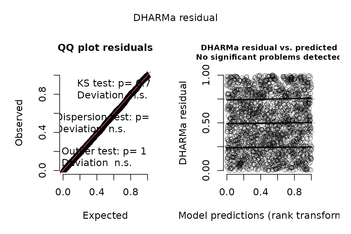

For random-intercept fits, simulate() draws fresh unit intercepts in every replicate, so the diagnostics are marginal over the random effects; see vignette("panels").

References

Dale, D. and Sirchenko, A. (2021). Estimation of nested and zero-inflated ordered probit models. Stata Journal, 21, 3-38.

Harris, M.N. and Zhao, X. (2007). A zero-inflated ordered probit model, with an application to modelling tobacco consumption. Journal of Econometrics, 141, 1073-1099.

King, G., Tomz, M. and Wittenberg, J. (2000). Making the most of statistical analyses: improving interpretation and presentation. American Journal of Political Science, 44, 347-361.

Krinsky, I. and Robb, A.L. (1986). On approximating the statistical properties of elasticities. Review of Economics and Statistics, 68, 715-719.

Benjamin E. Bagozzi