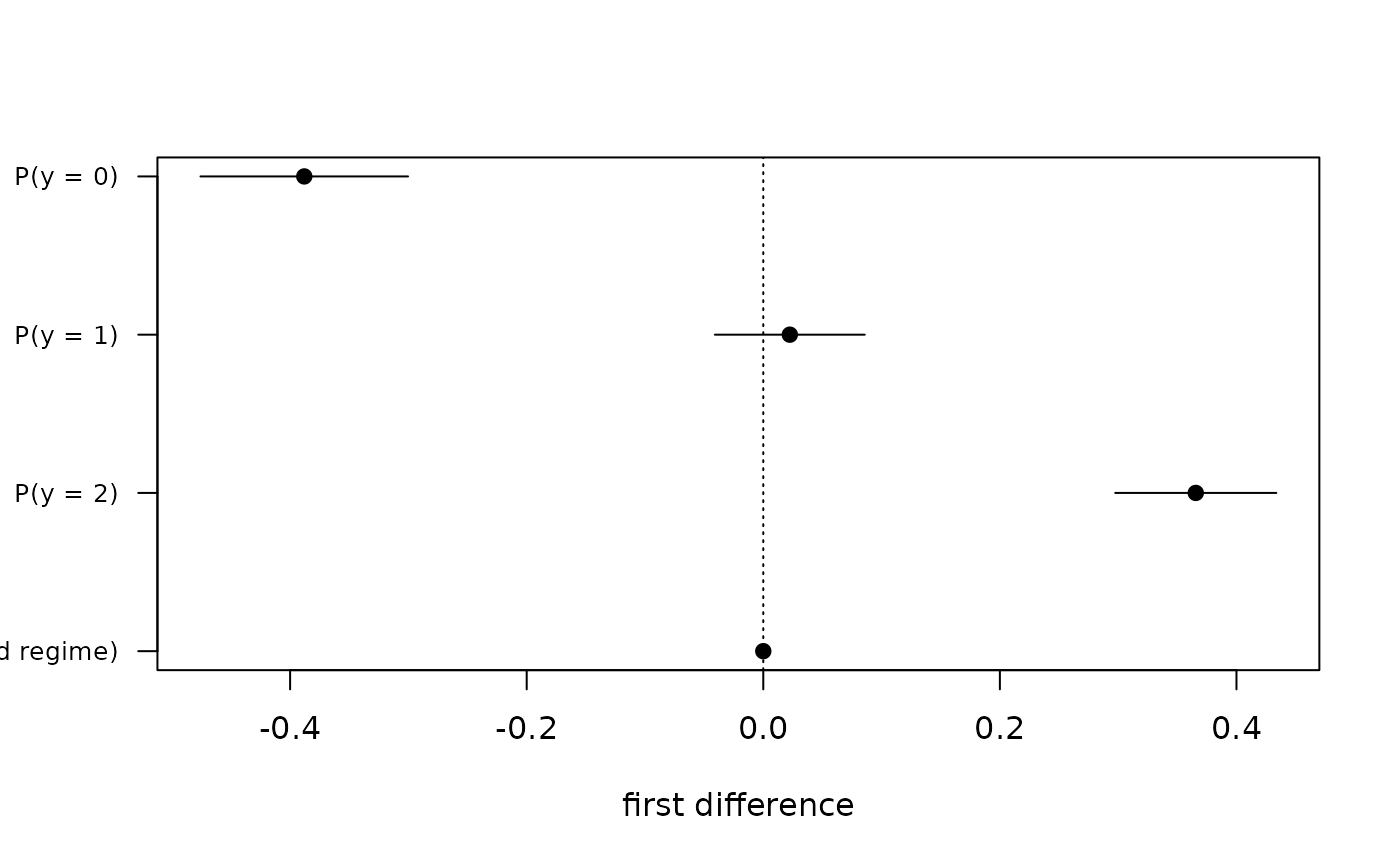
First differences in predicted probabilities

The change in each category probability \(P(y = j)\) – and, for inflated models, in the ordered-regime probability \(P(s = 1)\) – when one covariate moves from from to to, holding the others at a profile (default: weighted means of numeric covariates and modal levels of factors) or averaging over every observation's own covariates (average = TRUE). For inflated models the covariate can be moved in both equations (the total effect), in the outcome equation only, or in the inflation equation only; a covariate absent from an equation simply has no effect there.

Usage

first_difference(
  object,
  var,
  from,
  to,
  newdata = NULL,
  average = FALSE,
  stage = c("both", "outcome", "inflation"),
  ci = c("delta", "sim", "none"),
  level = 0.95,
  R = 1000,
  decompose = FALSE,
  ...
)

Arguments

object: An "iord" object.
var: Name of the covariate to move.
from, to: Its two values (numbers, or level labels for a factor).
newdata: Optional one-row data frame giving the profile of the other covariates; default is the typical profile described above. For a fixed-effects fit the default profile sits at the modal unit (ties go to the first level); average = TRUE evaluates every unit at its own fixed effect, which is usually the more natural summary there. For a random-intercept fit the probabilities are marginal over the intercept.
average: If TRUE, average the first difference over the estimation data (each observation keeps its own other covariates); newdata is then ignored.
stage: For inflated models: "both" (default), "outcome", or "inflation".
ci: "delta" (default), "sim", or "none".
level: Confidence level.
R: Number of simulation draws when ci = "sim".
decompose: For inflated models, also report the change in the two components of the inflated-category probability – through the inflation process and through the ordered stage (see predict(type = "zeros")), the decomposition of Harris and Zhao (2007).
...: Unused; unknown arguments are an error.

Value

A data frame of class c("iop_fd", "data.frame") with one row per category (and one for P(ordered regime) in inflated models – one per non-inflated category under a category-specific split – plus the two components of the inflated-category probability when decompose = TRUE): component, from, to, diff, lower, upper, method.

Details

Intervals are by the delta method (analytic gradient of the probabilities with respect to the parameters, from the fitted covariance) or by simulation (R draws of the parameters from their asymptotic normal distribution, percentile bounds; Krinsky and Robb 1986; King, Tomz and Wittenberg 2000).

References

King, G., Tomz, M. and Wittenberg, J. (2000). Making the most of statistical analyses: improving interpretation and presentation. American Journal of Political Science, 44, 347-361. Harris, M.N. and Zhao, X. (2007). A zero-inflated ordered probit model, with an application to modelling tobacco consumption. Journal of Econometrics, 141, 1073-1099.

Examples

set.seed(7)
d <- riop(600, beta = c(0.8, -0.5), tau = c(-0.6, 0.7), gamma = c(0.3, 1), inflate = "bottom")
m <- iop(y ~ x1 + x2 | z1, d, inflate = "bottom")
first_difference(m, "x1", from = -1, to = 1)
#> First differences: x1 from -1 to 1 [at the typical profile]
#>          component  from    to   diff  lower  upper method
#>           P(y = 0) 0.741 0.353 -0.388 -0.476 -0.300  delta
#>           P(y = 1) 0.223 0.246  0.022 -0.041  0.086  delta
#>           P(y = 2) 0.036 0.402  0.366  0.298  0.434  delta
#>  P(ordered regime) 0.693 0.693  0.000  0.000  0.000  delta
first_difference(m, "z1", from = -1, to = 1, stage = "inflation", average = TRUE)
#> First differences: z1 from -1 to 1 (inflation equation only) [averaged over the estimation data]
#>          component  from    to   diff  lower  upper method
#>           P(y = 0) 0.821 0.375 -0.446 -0.519 -0.373  delta
#>           P(y = 1) 0.093 0.323  0.231  0.183  0.278  delta
#>           P(y = 2) 0.086 0.302  0.215  0.174  0.257  delta
#>  P(ordered regime) 0.269 0.940  0.671  0.567  0.774  delta
first_difference(m, "z1", from = -1, to = 1, decompose = TRUE)     # the two types of zeros
#> First differences: z1 from -1 to 1 [at the typical profile]
#>            component  from    to   diff  lower  upper method
#>             P(y = 0) 0.802 0.309 -0.493 -0.578 -0.408  delta
#>             P(y = 1) 0.131 0.457  0.326  0.258  0.395  delta
#>             P(y = 2) 0.067 0.234  0.167  0.125  0.209  delta
#>    P(ordered regime) 0.269 0.940  0.671  0.567  0.774  delta
#>  P(y = 0: inflation) 0.731 0.060 -0.671 -0.774 -0.567  delta
#>    P(y = 0: ordered) 0.071 0.249  0.178  0.111  0.245  delta
plot(first_difference(m, "x1", from = -1, to = 1))